(Note: This report was written as part of a computer vision course I took in 2017. I figured I’d post it here to share. Image above from Wikipedia)

Presented below are the results and discussion of my implementation of a simple Sum Squared Difference and advance energy minimization stereo algorithm (Census Transform with Semi-Global Matching), observing performance with respect to accuracy and runtime, and comparing their results against two state of the art stereo algorithms: ELAS and SGBM.

1. Introduction

Stereo algorithms can be generally divided into four steps based on the taxonomy proposed in 2002 by Scharstein and Szeliski [1]: matching cost computation, cost aggregation, disparity selection, and disparity refinement. The figure shown below from Hamzah and Ibrahim [2] helps to provide some context:

The first two steps, matching cost and cost aggregation, will be most relevant to the following discussion. The algorithms were evaluated following the format of the Middlebury Stereo Evaluation suite (vision.middlebury.edu/stereo).

For the remainder of this report, I will briefly summarize the stereo algorithms I’ve implemented in Section 2. The disparity images resulting from these algorithms are presented in Section 3, along with results from two state of the art methods for comparison (ELAS and SGBM). The aggregated statistics for accuracy and runtime for each algorithm are presented in Section 4. A technical discussion of the algorithm results is presented in Section 5. A full list of references to research papers and other articles is provided in Section 6.

2. Descripton of Algorithms Implemented

Matching cost is the step of the stereo correspondence pipeline responsible for assigning a “score” to a proposed pixel match from a base image $I_b$ to a match image $I_m$ for some proposed disparity $d$. The way these scores are assigned depend on the matching cost algorithm selected – in this case the SSD and CT algorithms were explored. Cost aggregation is a subsequent step in which an algorithm processes the matching cost $C$ and can enforce additional constraints, formulating the disparity selection into a global energy minimization problem.

2.1 Sum Squared Difference (SSD)

Determining the matching cost of a rectified stereo pair of images $I_b$ and $I_m$ using SSD can be done simply with the following steps:

• Allocate a 3D matrix $C$ of size ($width$, $height$, $maxdisp+1$), with $maxdisp$ being the max disparity value to search for matches up to.
• For each proposed disparity, $d = 0$ to $maxdisp$:
  • Shift the match image $I_m$ by $d$ pixels along the epipolar line (i.e. the horizontal axis)
  • Subtract the shifted match image from the base image $I_b$, and then square those values resulting in a “squared difference” image
  • Use a kernel (or window) to filter over the image and “sum” the values within the window to be stored in a new image, the “sum squared difference”
  • Store the “sum squared difference” image as the $d$-th layer of $C$

The disparity map can then be calculated by $\underset{d}{\operatorname{argmin}} C(i,j,d)$. There is no following cost aggregation step, nor any disparity refinement in this case.

2.2 Census Transform (CT)

The Rank and Census Transforms were introduced in 1994 by Zabhi and Woodfill [4] as a non-parametric local transform. The Census Transform encodes its local neighborhood about a center pixel as a bitstring, where each value in the bitstring is simply whether the intensity of the neighboring pixel is less than intensity of the center pixel. If neighbor pixel intensity is less than the center pixel, assign a value of 0, else 1. Below is a simple example of calculating a single pixel’s bitstring using a 3x3 window, taken from the web [6]:

Because it’s representation is independent of the actual intensity value of its neighbors (only the intensity relative to the center), Census Transform is tolerant to changes to scene intensity between the base and match images such as different lighting conditions. Additionally, it has strong performance near object borders compared to simpler methods such as SSD [5]. After calculating the representative bitstrings of each pixel in $I_b$ and $I_m$, given as $\bar{I}_b$ and $\bar{I}_m$ respectively, populating the 3D cost matrix $C$ is done with the following steps:

• Allocate a 3D matrix $C$ of size ($width$, $height$, $maxdisp+1$), with $maxdisp$ being the max disparity value to search for matches up to.

• For each proposed disparity, $d = 0$ to $maxdisp$:

  • Shift the match census image: $\bar{I}_{m}$ by $d$ pixels
  • Let this be called $\bar{I}_{m,d}$
  • Calculate the Hamming distance between the bitstring values at each pixel:
  • $C[i,j,d] = Hamming(\bar{I}_{m,d}(i,j), \bar{I}_b(i,j))$

Where the Hamming distance is the count of the number of positions where the bitstrings differ. From my experimentation, the disparity map that results from simply calling $\underset{d}{\operatorname{argmin}} C(i,j,d)$ when using Census Transform results in poor accuracy. Pairing this matching cost matrix $C$ with SGM, however, leads to quite good results (as covered in Section 3).

2.3 Semi-Global Matching (SGM)

Global stereo algorithms (as opposed to local ones, such as SSD) typically make an assumption of smoothness about the disparity image and use optimization to minimize the overall energy $E$ for some proposed disparity map $D$. For SGM, the energy $E(D)$ that depends on the disparity image $D$ is given by the following equation from [3]:

\[E(D) = \sum\limits_{p}(C(p,D_p) + \sum\limits_{q \in N_p} P_1 T[|D_p - D_q| = 1] + \sum\limits_{q \in N_p} P_2 T [|D_p - D_q| > 1])\]

The 2D global minimization given above is unfortunately NP-complete [3]. To address this, SGM introduces it’s novel “path-wise aggregation” which does minimization along multiple 1D image rows symmetrically about every pixel, which approximates the 2D global minimization in polynomial time.

The cost (or energy) along a path $\textbf{r}$ is given by $L_{\textbf{r}}$ for some pixel $\textbf{p}$ at proposed disparity $d$:

\[\begin{aligned} L_{\textbf{r}}(\textbf{p}, d) = & C(\textbf{p},d) + \min(L_{\textbf{r}}(\textbf{p}-\textbf{r},d), \\ & \hspace{6.5em} L_{\textbf{r}}(\textbf{p}-\textbf{r}, d-1) + P_1, \\ & \hspace{6.5em} L_{\textbf{r}}(\textbf{p}-\textbf{r}, d+1) + P_1, \\ & \hspace{6.5em} \min\limits_{i} L_{\textbf{r}} (\textbf{p}-\textbf{r},i) + P_2) \\ & \hspace{3.25em} - \min\limits_{k} L_{\textbf{r}} (\textbf{p}-\textbf{r}, k) \end{aligned}\]

This algorithm is used starting from the border and recursively calculates the cost along the path towards pixel $\textbf{p}$. Next, the aggregated (or “smoothed”) cost for pixel $\textbf{p}$ and disparity $d$ is calculated as the sum across all paths $L_{\textbf{r}}$: \(S(\textbf{p}, d) = \sum\limits_{\textbf{r}} L_{\textbf{r}} (\textbf{p}, d)\)

The disparity map is then calculated by $\underset{d}{\operatorname{argmin}} S(i,j,d)$, where additional refinement to the disparity map may follow.

2.4 CT-SGM

In the 2008 presentation of SGM by Heiko Hirschmüler[3], Mutual Information was used as the matching cost algorithm. In my experimentation, using Absolute Difference (AD) as matching cost with SGM was attempted, but the results of AD-SGM were not significantly better (and sometimes worse) than SSD.

Census Transform, while not “cutting edge” in terms of how recently it was introduced, has been shown to perform quite well even compared to MI and other state of the art matching cost algorithms in 2008 [5]. Because of its indicated strong performance and straight-forward algorithm, it was selected to be the matching cost algorithm which feeds into SGM, hence CT-SGM.

Some other key differences between my implementation and the original SGM:

• Hirschmüler’s original SGM employed a hierarchical pattern, starting with input images downsampled by a scale factor $s$, looping through the entire pipeline until $s = 1$. In contrast, my CT-SGM implementation is made up of only a single pass, with only a 3x3 median blur as disparity refinement.
• Original SGM aggregates over 16 paths, while my implementation supports only 4 paths (up, down, left, right) or 8 paths (includes diagonals).

A summary of the steps in my CT-SGM algorithm are expressed below: \(CT(I_b, I_m) => C_{CT} => S_{SGM} => \underset{d}{\operatorname{argmin}}S_{SGM} => D\prime => medianblur(D\prime) => D\)

3. Results

Presented here are the results of my algorithms alongside state of the art reference implementations, ELAS and OpenCV SGBM. SGBM is an implementation of SGM that utilizes the Birchfield and Tomasi (BT) matching cost algorithm with “block matching” (as opposed to pixel-wise). My methods are labeled pvp-ssd, pvp-ctsgm4, and pvp-ctsgm8, where 4 and 8 denote the number of paths for the aggregation step. While my implementations provide both a “left-to-right” (L) and a “right-to-left” (R) disparity image, these are omitted in for ELAS and SGBM. The metrics of interest below are:

• bad0.5 is the percentage of pixels whose disparity is more than 0.5 pixels off from the ground truth disparity map. Lower bad0.5 is better.
• runtime is simply how long it took for my computer to process the disparity map (in seconds).

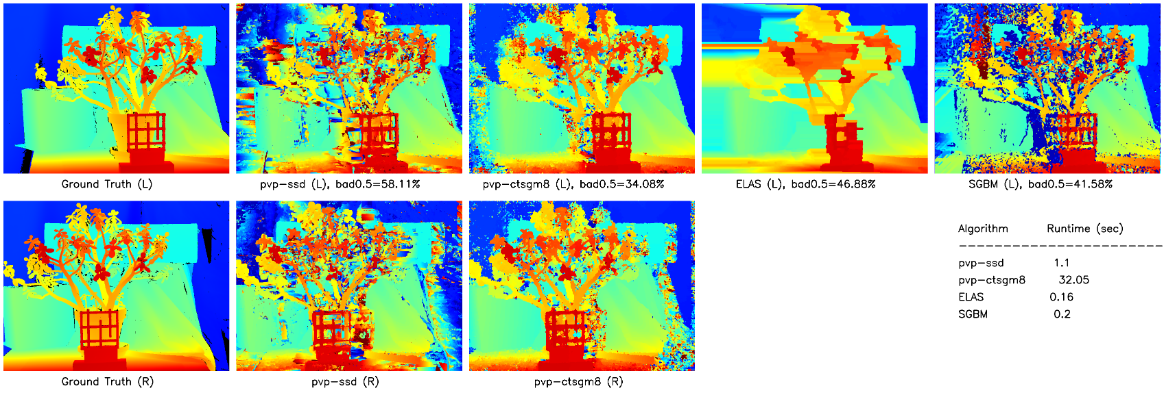
The Jadeplant dataset (Fig 4) has a large number of fine features, which is problematic for ELAS as it appears to smooth the disparity map quite agressively. CT-SGM outperforms the other algorithms in this case, with SSD lagging behind but outputting a decent looking disparity map.

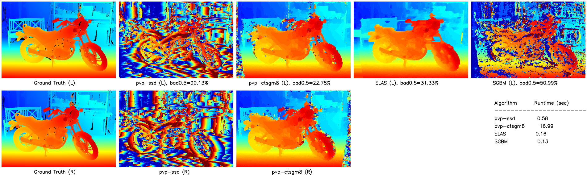
For the MotorcycleE dataset (Fig 5), SSD and SGBM accuracies degrade with respect to the the Motorcycle dataset due to a difference in illumination of the scene between the left and right images (not pictured). Changes in illumination, or more broadly radiometric differences, cause major problems for local matching costs that do not use normalization (such as Normalized Cross Correlation, NCC). CT-SGM and ELAS, on the other hand, still perform well (in fact, CT-SGM scores a higher accuracy with the illumination difference than without!).

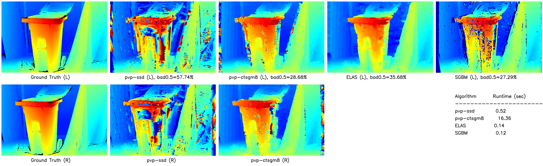
The Recycle dataset (Fig 6) showcases another drawback of SSD (and Sum Absolute Difference, SAD, for the same reason): there is no unique minimum on a large region of uniform shading or periodic pattern [7]. SGBM proves to perform the best on this dataset by a small margin.

4. Performance Statistics

The Middlebury Stereo Evaluation uses test datasets (with ground truth hidden) and weights certain sets more strongly than others for an aggregated score. For this discussion, we will consider only the set of 15 “Quarter sized” training datasets and weight them all equally. Recalling that pvp-ctsgm4 is the same CT-SGM that aggregates over 4 paths instead of 8, the average performance of each of the considered algorithms is calculated to be:

Algorithm	bad0.5 (%)	avgErr (%)	Runtime (sec)
ELAS	37.76	2.18	0.14
SGBM	38.02	6.62	0.13
pvp-ctsgm4	34.66	2.41	11.21
pvp-ctsgm8	34.26	2.31	17.34
pvp-ssd	61.66	7.52	0.58

A technical discussion of table above follows in the next section.

5. Technical Discussion of Results

From the table above, we see that the CT-SGM algorithms actually outperform ELAS and SGBM in the bad0.5 metric by a small margin (3% to 4%), while SSD performs far worse. We notice immediately, however, that the runtime performance of the reference implementations are more than two orders of magnitude faster than CT-SGM.

Part of the reason for this is that the reference implementations have been written in C++ and have almost certainly been highly optimized for performance. Conversely, the CT-SGM code is written in Python and is relatively unoptimized aside from using some NumPy vectorization. As a point of reference, ELAS is currently ranked 4th and SGBM ranked 8th under the “time/MP” metric on Middlebury Stereo Evaluation (MSE) page, which measures the runtime (in seconds) normalized by pixels processed (in mega-pixels).

To improve upon my modified SGM algorithm, a more suitable matching cost algorithm could be selected to pair with SGM (with a preference for improving runtime). The obvious next matching cost to try would be MI, as originally proposed. Other matching cost functions which could show promise are Zero-mean Normalized Cross Correlation (ZNCC) and the Birchfield and Tomasi (BT) matching cost (also referenced in [3]).

With regard to runtime performance, the option to rewrite the code in C++ is available. However, there are likely additional NumPy optimizations which could improve runtime of my code, which would likely be the least expensive way improve runtime performance. When a wall is reached in NumPy optimization, slower parts of the algorithm could be compiled to C using a Just-in-Time (JIT) Python compiler such as Numba. Restructuring of the code to run in a highly parallelized fashion on a GPU would also make for a fun challenge: one popular library for this is PyCUDA. Further extensions of SGM from more recent publications which should be explored are Iterative SGM (iSGM)[8] and Weighted SGM (wSGM)[9].

6. References

• [1] Scharstein and Szeliski, 2002, A Taxonomy and Evaluation of Dense Two-Frame Stereo Correspondence Algorithms
• [2] Hamzah and Ibrahim, 2015, Literature Survey on Stereo Vision Disparity Map Algorithms
• [3] Hirschmüler, 2008, Stereo Processing by Semi-Global Matching and Mutual Information
• [4] Zabih and Woodfill, 1994, Non-parametric Local Transforms for Computing Visual Correspondence
• [5] Hirschmüler and Scharstein, 2008, Evaluation of Stereo Matching Costs on Images with Radiometric Differences
• [6] Intel Developer Zone: Census Transform Algorithm Overview
• [7] Klette, 2014, Concise Computer Vision: An Introduction into Theory and Algorithms
• [8] Hermann and Klette, 2012, Iterative Semi-Global Matching for Robust Driver Assistance Systems
• [9] Spangenberg, Langner, and Rojas, 2013, Weighted Semi-Global Matching and Center-Symmetric Census Transform for Robust Driver Assistance