
The Draughtsmen of the Lute by Albrecht Dürer (The Met).
Table of Contents:
- Intro
- What is camera calibration?
- Camera parameters: A, W, k
- Projection: from 3D world point to 2D image point
- Aside: detecting target points in 2D images
- (Re)projection error: E
- Up next…
- Appendix
Intro
Below is a primer on the theory behind camera calibration. Zhang’s method specifically will be covered in part 2. My hope is that the ordering of concepts here will help new readers feel at home more quickly when navigating calibration literature.
For a deep dive into Zhang’s method, I highly recommend this tutorial paper by Burger. I’ve also written a heavily commented Python implementation: github.com/pvphan/camera-calibration.
And here’s an image which helps paint a picture of the information considered in camera calibration:
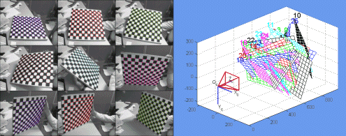
A calibration dataset and its ‘camera centric’ board pose visualization (vision.caltech.edu).
What is camera calibration?
A camera captures light from a 3D world and projects it onto a 2D sensor which stores the sensor state as a 2D image. In other words, a 2D point in the image is equivalent to a 3D ray in the scene. A camera is calibrated if we know the camera parameters which define the mapping between these spaces.
Camera calibration is the process of computing the camera parameters: \(A\), \(\textbf{W}\), and \(\textbf{k}\). These are further discussed just below in the \(\S\)camera parameters section.
A camera calibration dataset is gathered by capturing multiple images of a known physical calibration target and varying the board pose with respect to the camera for each view.
So, given multiple images of a known calibration target, camera calibration computes the camera parameters: \(A\), \(\textbf{W}\), and \(\textbf{k}\). And with these parameters, we can reason spatially about the world from images!
Camera parameters: A, W, k
You’ll have to bear with these largely unmotivated definitions for a moment. I wanted them laid out plainly here in one spot, and their use will be explained in the next section on \(\S\)projection.
- \(A\) — the intrinsic matrix,
\(\begin{pmatrix}
\alpha & \gamma & u_0\\
0 & \beta & v_0\\
0 & 0 & 1\\
\end{pmatrix}\)
- \(\alpha\) — focal length in the camera x direction
- \(\beta\) — focal length in the camera y direction
- \(\gamma\) — the skew ratio, typically 0
- \(u_0\) — u coordinate of optical center in image coordinates
- \(v_0\) — v coordinate of optical center in image coordinates
- In other literature, the intrinsic matrix \(A\) is often denoted \(\textbf{K}\), \(\alpha\) as \(f_x\), \(\beta\) as \(f_y\), etc
- \(\textbf{W}\) — the per-view set of transforms (also called extrinsic parameters) from world to camera, which is a list of N 4x4 matrices
- \(\textbf{W} = [W_1, W_2, ..., W_n]\), where \(W_i\) is the \(i\)-th rigid-body transform from world to camera, which is also the pose of the world in camera coordinates (see the \(\S\)appendix for more discussion on convention)
- Here, and in other literature, the coordinate frame of the calibration board is called the world coordinate frame. All of these coordinate frames are equivalent in this post: world \(=\) target $=$ calibration board
- \(\textbf{k}\) — the distortion vector:
\(\begin{pmatrix}
k_1 & k_2 & p_1 & p_2 & k_3
\end{pmatrix}\)
- \(k_i\) values correspond to radial distortion and \(p_i\) values correspond to tangential distortion (for the so-call radial-tangential distortion model)
Projection: from 3D world point to 2D image point
The journey of a 3D world point to a 2D image point is a series of four transformations, corresponding almost one-to-one with the calibration parameters \(A\), \(\textbf{W}\), and \(\textbf{k}\) we are solving for. Each step has an equation in it’s compact form (X.a) and in more verbose form (X.b).
A quick summary of the journey:
- Rigidly transform 3D points in world coordinates to 3D camera coordinates with \(\textbf{W}\).
- Project these 3D points into the cameras 2D ‘normalized plane’ (\(z = 1\)).
- Distort the normalized 2D points by the distortion model and parameters \(\textbf{k}\).
- Project the distorted-normalized points into the 2D image coordinates with the intrinsic matrix \(A\).
We’ll call each step Proj.<N> to disambiguate with the steps of Zhang’s method in part 2.
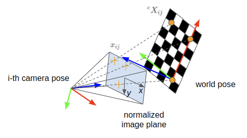
Proj.1) Use \(\textbf{W}\): 3D world point to 3D camera point
![]()
This is a simple one for those already familiar with 3D coordinate transformations. We begin with a 3D point in world coordinates, expressed as \({}^wX_{ij}\). Here (and following), \(i\) refers to which image a variable corresponds to, and \(j\) refers to the point instance within that image.
\[\begin{equation} {}^cX_{ij} = W_i \cdot {}^wX_{ij} \tag{1.a}\label{eq:1.a} \end{equation}\] \[\begin{equation} \begin{pmatrix} x_c\\ y_c\\ z_c\\ 1\\ \end{pmatrix} _{ij} = \begin{pmatrix} | & | & | & t_x\\ r_{x} & r_{y} & r_{z} & t_y\\ | & | & | & t_z\\ 0 & 0 & 0 & 1\\ \end{pmatrix} _{i} \begin{pmatrix} x_w\\ y_w\\ z_w\\ 1\\ \end{pmatrix} _{ij} \tag{1.b}\label{eq:1.b} \end{equation}\]- \({}^cX_{ij}\) — the \(j\)-th 3D point in camera coordinates from the \(i\)-th image, given in homogeneous coordinates
- \(W_i\) — the transform from world coordinates to camera coordinates for the \(i\)-th image
- \({}^wX_{ij}\) — the \(j\)-th 3D point in world coordinates, given in homogeneous coordinates
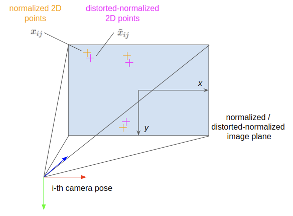
Proj.2) Use \(\Pi\): 3D camera coordinates to 2D normalized image point
Next we’ll project the 3D coordinate in the cameras frame into the normalized image plane. This is done by intersecting the ray from optical center to that 3D point with the \(z = 1\) plane.
\[\begin{equation} x_{ij} = hom^{-1}(\Pi \cdot {}^cX_{ij}) \tag{2.a}\label{eq:2.a} \end{equation}\] \[\begin{equation} \begin{pmatrix} x\\ y\\ \end{pmatrix} _{ij} = hom^{-1} \left( \begin{pmatrix} 1 & 0 & 0 & 0\\ 0 & 1 & 0 & 0\\ 0 & 0 & 1 & 0\\ \end{pmatrix} \begin{pmatrix} x_c\\ y_c\\ z_c\\ 1\\ \end{pmatrix} _{ij} \right) \tag{2.b}\label{eq:2.b} \end{equation}\]- \(x_{ij}\) — the 2D projected coordinate of the point in the normalized image
- \(x\) — the x component of the normalized 2D point
- \(y\) — the y component of the normalized 2D point
- \(hom^{-1}(\cdot)\) — the function which maps a homogeneous coordinate to its unhomogeneous equivalent point (divide the vector by its last value, then drop the trailing 1)
- \(\Pi\) — the ‘standard projection matrix’ which reduces the dimensionality
In other literature, it’s common to express the projection of a 3D point in camera onto the normalized image plane by simply dividing the point in camera coordinates by it’s \(z\) component and dropping the \(z\) term:
\[\begin{pmatrix} x\\ y\\ \end{pmatrix} = \begin{pmatrix} x_c/z_c\\ y_c/z_c\\ \end{pmatrix}\]But I prefer the matrix multiplication and \(hom^{-1}(\cdot)\) presented previously for continuity of equations.
Proj.3) Use \(\textbf{k}\): 2D normalized point to 2D distorted-normalized point
This step accounts for lens distortion by applying a non-linear warping function in normalized image coordinates. We’ll call the resulting point a ‘distorted-normalized’ point since it’s still in the normalized space, but has had lens distortion applied to it.
\[\begin{equation} \tilde{x}_{ij} = distort(x_{ij}, \textbf{k}) \tag{3.a}\label{eq:3.a} \end{equation}\] \[\begin{equation} \begin{pmatrix} \tilde{x}\\ \tilde{y}\\ \end{pmatrix} _{ij} = \begin{pmatrix} d_{radi} x + d_{tang,x}\\ d_{radi} y + d_{tang,y}\\ \end{pmatrix} _{ij} \tag{3.b}\label{eq:3.b} \end{equation}\] \[d_{radi} = (1 + k_1 r^2 + k_2 r^4 + k_3 r^6)\] \[d_{tang,x} = 2 p_1 x y + p_2 (r^2 + 2 x^2)\] \[d_{tang,y} = p_1 (r^2 + 2 y^2) + 2 p_2 x y\] \[r = \sqrt{x^2 + y^2}\]- \(\tilde{x}_{ij}\) — the 2D distorted-normalized point
- \(\tilde{x}\) — the distorted-normalized point, x component
- \(\tilde{y}\) — the distorted-normalized point, y component
- \(\textbf{k}\) — the distortion vector, \((k_1, k_2, p_1, p_2, k_3)\)
- \(r\) — the radial distance the 2D normalized point is from the optical center \((0, 0)\)
- \(d_{radi}, d_{tang,x}, d_{tang,y}\) — the radial, tangential (x), and tangential (y) effects on the final distorted-normalized point
The \(distort(\cdot)\) function here is dependent upon the selected lens distortion model. Here we use the popular radial-tangential distortion model (also called the Plumb Bob or Brown-Conrady model (source: calib.io)).
Proj.4) Use \(A\): 2D distorted-normalized point to 2D image point
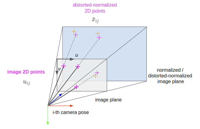
At last, we can project the distorted rays of light into our image plane. Points in the image plane have coordinates \(u_{ij}\) and are in units of pixels, with the origin starting in the top-left of the image. The value \(u\) increases from left-to-right, and \(v\) increases from top-to-bottom of the image.
\[\begin{equation} u_{ij} = hom^{-1}(A \cdot hom(\tilde{x}_{ij})) \tag{4.a}\label{eq:4.a} \end{equation}\] \[\begin{equation} \begin{pmatrix} u\\ v\\ \end{pmatrix} _{ij} = hom^{-1} \left( \begin{pmatrix} \alpha & \gamma & u_0\\ 0 & \beta & v_0\\ 0 & 0 & 1\\ \end{pmatrix} \begin{pmatrix} \tilde{x}\\ \tilde{y}\\ 1\\ \end{pmatrix} _{ij} \right) \tag{4.b}\label{eq:4.b} \end{equation}\]- \(u_{ij}\) — the 2D image point
- \(u\) — the horizontal component of the image point
- \(v\) — the vertical component of the image point
- \(A\) — the intrinsic matrix
- \(hom(\cdot)\) — the function which maps an unhomogeneous point to it’s homogeneous equivalent (for a 2D point, append a 1 to the end of the vector)
The rest of the variables have been previously described in the \(\S\)camera parameters section and won’t be repeated here.
Beware that some linear algebra libraries (e.g. numpy) index in ‘row, column’ order.
So accessing a value of \(u, v\) would be done via value = image[v, u].
All together!
Combining the above four steps, we can express projection more compactly as a function of inputs and calibration parameters:
\[\begin{equation} u_{ij} = \underbrace{hom^{-1} ( A \cdot hom( \underbrace{distort( \underbrace{hom^{-1}( \Pi \cdot \underbrace{W_i \cdot {}^wX_{ij}}_\textrm{Proj.1: ${}^cX_{ij}$} )}_\textrm{Proj.2: $x_{ij}$}, \textbf{k} )}_\textrm{Proj.3: $\tilde{x}_{ij}$} ) )}_\textrm{Proj.4: $u_{ij}$} \tag{5}\label{eq:5} \end{equation}\]We’ve now defined a basis for predicting where a point will be in our image provided we have a known target point \({}^wX_{ij}\) and values for the calibration parameters \(A, W_i, \textbf{k}\).
But how do we measure (or detect) the 2D points from the images in our dataset?
Aside: detecting target points in 2D images
For the remainder of this post, we will assume the 2D target points (in pixel coordinates) have already been detected in the images and have known association with the 3D target points in the target’s coordinate system. Such functionality is typically handled by a library (e.g. ChArUco, AprilTag) and is beyond the scope of this post.
Such libraries typically detect strong corners made unique by specific neighboring patterns, or detect circle centers which have a unique distribution of small vs large circles.

The corners of the larger checkerboard are the points which are detected (OpenCV.org).
And with that, we’re ready to talk about projection error (sometimes called reprojection error).
(Re)projection error: E
In order to compute camera parameters which are useful for spatial reasoning, we need to define what makes one set of parameters better than another set. This is typically done by computing sum-squared projection error, \(E\). The lower that error metric is, the more closely our camera parameters fit the measurements from the input images.
- From each image, we have the detected marker points. Each marker point is a single 2D measurement, which we denote as \(z_{ij}\) for the \(j\)-th measured point of the \(i\)-th image.
- From each measurement \(z_{ij}\), we also have the corresponding 3D point in target coordinates \({}^wX_{ij}\) (known by construction).
- With a set of calibration parameters (\(A\), \(W_i\), \(\textbf{k}\)), we can then project where that 3D point should appear in the 2D image — a single 2D prediction, which we express as the image point, \(u_{ij}\).
- The Euclidean distance between the 2D prediction and 2D measurement is the projection error for a single point.
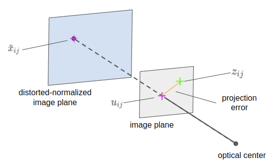
Illustration of projection error for a single measurement (\(z_{ij}\)) and prediction (\(u_{ij}\)).
Considering the full dataset, we can compute the sum-squared projection error by computing the Euclidean distance (also called the L2-norm, denoted \(|| \cdot ||\) ) between each measurement-prediction pair for all $n$ images and all $m$ points in those images:
\[\begin{equation} E = \sum\limits_{i}^{n} \sum\limits_{j}^{m} || z_{ij} - u_{ij} ||^2 \tag{6}\label{eq:6} \end{equation}\]where the Euclidean distance between vectors \(p\) and \(q\) (each of length \(l\)) is a scalar value defined as:
\[\begin{equation} || p - q || = \sqrt{\sum\limits_{k}^{l} (p_k - q_k)^2} \tag{7}\label{eq:7} \end{equation}\]Now we have a way to compute how closely our calibration parameters and measurements match — the ‘goodness’ of the calibration. But how do we get values for these calibration parameters?
Up next…
In Part 2 of this post we’ll get into Zhang’s method, currently the most popular way to calibrate cameras due to it’s accessibility and accuracy. It requires only a planar calibration target which can be made with any desktop printer.
Special thanks to my co-worker @RajRavi for feedback on this post.
Appendix
Rigid-body transformations
Recall we defined \(\textbf{W} = [W_1, W_2, ..., W_n]\), where \(W_i\) is the \(i\)-th rigid-body transform from world to camera, which is also the pose of the world in camera coordinates.
This can also be written in what I’ve been told is the ‘Craig convention’: \(\textbf{W} = [{}^cM_{w,1}, {}^cM_{w,2}, ..., {}^cM_{w,N}]\), where \({}^cM_{w,i}\) is the \(i\)-th rigid-body transform from world to camera, which is also the pose of the world in camera coordinates.
Each transform expressed in homogeneous form:
\[{}^cM_{w} = \begin{pmatrix} | & | & | & t_x\\ r_{x} & r_{y} & r_{z} & t_y\\ | & | & | & t_z\\ 0 & 0 & 0 & 1\\ \end{pmatrix}\]- \(t_x, t_y, t_z\) are the world coordinate system’s origin given in the camera’s coordinates
- \(r_x\) (3x1 column vector) is the normalized direction vector of the world coordinate system’s x-axis given in the camera’s coordinates (\(r_y\), \(r_z\) follow this pattern)
Notational example of transforming a single, homogeneous 3D point:
\[{}^cP = {}^cM_{w} \cdot {}^wP\] \[P \in \mathbb{R^3}\] \[{}^cM_{w} \in SE(3)\]-
\({}^cP\) — homogeneous point \(P\) in camera coordinates, \(\begin{pmatrix} x_c & y_c & z_c & 1 \end{pmatrix} ^\top\)
-
\({}^wP\) — homogeneous point \(P\) in world coordinates, \(\begin{pmatrix} x_w & y_w & z_w & 1 \end{pmatrix} ^\top\)
- \(\mathbb{R^3}\) — the space of real, 3 dimensional numbers
- \(SE(3)\) — \(S\)pecial \(E\)uclidean group 3, the space of 3D rigid-body transformations