School of Athens by Raphael (Musei Vaticani).

Table of Contents:

• Intro
• What is ‘Zhang’s method’?
  • Intuition by dependency graph
• The steps of Zhang’s method
  • Zhang.1) Homography estimation using Direct Linear Transformation (DLT)
    • Relate world points to image points as homographies, \(H_i\)
    • Reformulate using DLT
    • Solve for \(\textbf{h}\) in \(M \cdot \textbf{h} = \textbf{0}\) using SVD
  • Zhang.2) Compute initial intrinsic matrix, \(A_{init}\)
    • Reformulate using DLT
    • Solve for \(b\) in \(V \cdot \textbf{b} = \textbf{0}\) using SVD
  • Zhang.3) Compute initial extrinsic parameters, \(W_{init}\)
  • Zhang.4) Compute initial distortion vector, \(k_{init}\)
  • Zhang.5) Refine A, W, k using non-linear optimization
• Final remarks
• Appendix
  • Singular Value Decomposition (SVD)
  • Non-linear least squares optimization (Levenberg-Marquardt)

Intro

** Notice: this post is still under construction! Incomplete sections will be called out at the beginning. In particular, Zhang.2 is about halfway done, and Zhang.4 is empty. **

In Part 1, we defined the calibration parameters \(A, \textbf{W}, \textbf{k}\) and sum-squared projection error, \(E\). We now move on to how to estimate and refine these calibration parameters so we can reason spatially with images from that camera.

For a more complete walkthrough of each step of Zhang’s method, I’ve again linked the excellent tutorial paper by Burger. I’ll also link again the ‘from scratch’ Python implementation I wrote here: github.com/pvphan/camera-calibration.

What is ‘Zhang’s method’?

Currently, the most popular method for calibrating a camera is Zhang’s method published in A Flexible New Technique for Camera Calibration by Zhengyou Zhang (1998). Older methods typically required a precisely made 3D calibration target or a mechanical system to precisely move the camera or target. In contrast, Zhang’s method requires only a 2D calibration target and only loose requirements on how the camera or target moves. This means that anyone with a desktop printer and a little time can accurately calibrate their camera!

The general strategy of Zhang’s method is to impose naïve assumptions as constraints to get an initial guess of calibration parameter values with singular value decomposition (SVD), then release those constraints and refine those guesses with non-linear least squares optimization.

The ordering of steps for Zhang’s method are:

1. Use the 2D-3D point associations to compute the per-view set of homographies \(\textbf{H}\).
2. Use the homographies \(\textbf{H}\) to compute an initial guess for the intrinsic matrix, \(A_{init}\).
3. Using the above, compute an initial guess for the camera pose (per-view) in target coordinates, \(\textbf{W}_{init}\).
4. Using the above, compute an initial guess for the distortion parameters, \(\textbf{k}_{init}\).
5. Initialize non-linear optimization with the initial guesses above and then iterate to minimize projection error, producing \(A_{final}\), \(\textbf{W}_{final}\), and \(\textbf{k}_{final}\).

Intuition by dependency graph

Before we dive into the steps of Zhang’s method, I’ll present a dependency graph to illustrate which quantities contribute to which. This graph will serve as a map to aid in navigating the symbols and steps of Zhang’s method.

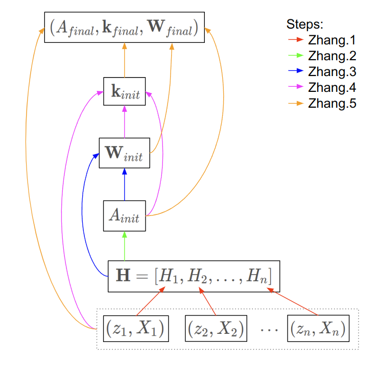
Here, the symbols \((z_i, X_i)\) represent the point detections for the \(i\)-th view, where \(z_i\) are the 2D point detections in the image and \(X_i\) are the corresponding 3D coordinates of those point in the calibration board’s coordinate frame.

The steps of Zhang’s method

Zhang.1) Homography estimation using Direct Linear Transformation (DLT)

Relate world points to image points as homographies, \(H_i\)

A homography is a 3-by-3 matrix that relates a plane in 3D space to another plane in 3D space. In our case, we care about the relation between the calibration board plane and the cameras sensor plane (assuming no lens distortion).

We will use the 2D-3D point associations to compute the homographies \(\textbf{H} = [H_1, H_2, ..., H_n]\), for each of the \(n\) views in the dataset. To do this we employ two tricks:

• Trick #1: Assume there is no distortion in the camera (7.a). This is of course not typically true, but it will let us compute approximate values to refine later.
• Trick #2: We define the world coordinate system so that it’s \(z = 0\) plane is the plane of the calibration target. This allows us to drop the \(z\) term of the 3D world points (7.b).

Trick #1 simplifies our projection equation (5) to a distortion-less pinhole camera model:

\[\begin{equation} u_{ij} = hom^{-1} ( A \cdot \Pi \cdot W_i \cdot {}^wX_{ij} ) \tag{7.a}\label{eq:7.a} \end{equation}\]

And after expanding, trick #2 allows us to drop some dimensions from this expression:

\[\begin{equation} \begin{bmatrix} u\\ v\\ 1\\ \end{bmatrix} _{ij} = hom^{-1} \left( A \cdot \begin{bmatrix} 1 & 0 & 0 & 0\\ 0 & 1 & 0 & 0\\ 0 & 0 & 1 & 0\\ \end{bmatrix} \begin{bmatrix} | & | & | & t_x\\ r_{x} & r_{y} & r_{z} & t_y\\ | & | & | & t_z\\ 0 & 0 & 0 & 1\\ \end{bmatrix} _{i} \begin{bmatrix} x_w\\ y_w\\ 0\\ 1\\ \end{bmatrix} _{ij} \right) \tag{7.b}\label{eq:7.b} \end{equation}\]

Now we can strike out the 3rd column of \(W_i\) and 3rd row of \({}^wX_{ij}\), and rewrite the \(hom^{-1}(\cdot)\) as a scale factor \(s\). We’ll call the product of \(A\) and that 3-by-3 matrix our homography, \(H_i\):

\[\begin{equation} s \begin{bmatrix} u\\ v\\ 1\\ \end{bmatrix} _{ij} = \underbrace{ A \cdot \begin{bmatrix} | & | & t_x\\ r_{x} & r_{y} & t_y\\ | & | & t_z\\ \end{bmatrix} _{i} }_{H_i} \begin{bmatrix} x_w\\ y_w\\ 1\\ \end{bmatrix} _{ij} \tag{8}\label{eq:8} \end{equation}\]

We’ll also shorthand the non-homogenous projected points \(s \cdot u\) to \(\hat{u}\), etc.

\[\begin{equation} s \begin{bmatrix} u\\ v\\ 1\\ \end{bmatrix} _{ij} = \begin{bmatrix} \hat{u}\\ \hat{v}\\ \hat{w}\\ \end{bmatrix} _{ij} \tag{9.a}\label{eq:9.a} \end{equation}\] \[\begin{equation} \begin{bmatrix} \hat{u}\\ \hat{v}\\ \hat{w}\\ \end{bmatrix} _{ij} = H_i \begin{bmatrix} x_w\\ y_w\\ 1\\ \end{bmatrix} _j \tag{9.b}\label{eq:9.b} \end{equation}\]

We’ve now arrived at an expression for our homography \(H_i\) which relates a 2D point on the target plane to a (non-homogeneous) 2D point on our image plane for the \(i\)-th view.

Reformulate using DLT

Next, we’ll use the Direct Linear Transformation (DLT) technique to rewrite this expression in homogeneous form \(M \cdot \textbf{h} = 0\). After that, we can apply Singular Value Decomposition (SVD) to solve for \(\textbf{h}\), and then reshape it into \(H\). To support a reformulation of (9.b), we define \(H_i\) and \(\textbf{h}_i\) as:

\[\begin{equation} H _{i} = \begin{bmatrix} h_{11} & h_{12} & h_{13} \\ h_{21} & h_{22} & h_{23} \\ h_{31} & h_{32} & h_{33} \\ \end{bmatrix} _{i} \tag{10}\label{eq:10} \end{equation}\] \[\begin{equation} \textbf{h}_i = \begin{bmatrix} h_{11} & h_{12} & h_{13} & \ h_{21} & h_{22} & h_{23} & \ h_{31} & h_{32} & h_{33} \end{bmatrix} _{i} ^\top \tag{11}\label{eq:11} \end{equation}\]

Now we’ll reformulate (9.b) so that we can solve for the values of \(H\). We desire an expression in terms of \(u\), \(v\), \(x_w\), and \(y_w\) (which are known) with respect to unknown values of \(\textbf{h}\) (which we will solve for).

Noting that \(s \equiv \hat{w}\) in equation (9.a), we can rewrite it as a pair of homogeneous equations:

\[\begin{equation} \left\{ \begin{aligned} u \hat{w} - \hat{u} = 0 \\ v \hat{w} - \hat{v} = 0 \end{aligned} \right. \tag{12}\label{eq:12} \end{equation}\]

And relating the second and third terms from (9.b) with the elements of \(H_i\) distributed:

\[\begin{equation} \begin{split} \hat{u} = h_{11} x_w + h_{12} y_w + h_{13} \\ \hat{v} = h_{21} x_w + h_{22} y_w + h_{23} \\ \hat{w} = h_{31} x_w + h_{32} y_w + h_{33} \\ \end{split} \tag{13}\label{eq:13} \end{equation}\]

Substituting (13) into (12) and reordering the terms by the elements of \(\textbf{h}_i\), we get:

\[\begin{equation} \left\{ \begin{aligned} - h_{11} \cdot x_w - h_{12} \cdot y_w - h_{13} + u \cdot h_{31} x_w + u \cdot h_{32} y_w + u \cdot h_{33} = 0 \\ - h_{21} \cdot x_w - h_{22} \cdot y_w - h_{23} + v \cdot h_{31} x_w + v \cdot h_{32} y_w + v \cdot h_{33} = 0 \end{aligned} \right. \tag{14}\label{eq:14} \end{equation}\]

Which for this pair of equations can be rewriten into matrix form as:

\[\begin{equation} \begin{bmatrix} - x_{w,j} & - y_{w,j} & -1 & 0 & 0 & 0 & u_j \cdot x_{w,j} & u_j \cdot y_{w,j} & u_j \\ 0 & 0 & 0 & - x_{w,j} & - y_{w,j} & -1 & v_j \cdot x_{w,j} & v_j \cdot y_{w,j} & v_j \\ \end{bmatrix} _{i} \begin{bmatrix} h_{11}\\ h_{12}\\ h_{13}\\ h_{21}\\ h_{22}\\ h_{23}\\ h_{31}\\ h_{32}\\ h_{33}\\ \end{bmatrix} _{i} = \begin{bmatrix} 0\\ 0\\ \end{bmatrix} \tag{15}\label{eq:15} \end{equation}\]

By iterating over each $j$-th point for \(j \in [1, 2, ..., m]\) and stacking these pairs of equations vertically, we create a matrix we’ll call \(M_i\) which relates each observed point in an image to it’s position in world coordinates by the quantity \(\textbf{h}_i\):

\[\begin{equation} \begin{bmatrix} - x_{w,1} & - y_{w,1} & -1 & 0 & 0 & 0 & u_1 \cdot x_{w,1} & u_1 \cdot y_{w,1} & u_1 \\ 0 & 0 & 0 & - x_{w,1} & - y_{w,1} & -1 & v_1 \cdot x_{w,1} & v_1 \cdot y_{w,1} & v_1 \\ - x_{w,2} & - y_{w,2} & -1 & 0 & 0 & 0 & u_2 \cdot x_{w,2} & u_2 \cdot y_{w,2} & u_2 \\ 0 & 0 & 0 & - x_{w,2} & - y_{w,2} & -1 & v_2 \cdot x_{w,2} & v_2 \cdot y_{w,2} & v_2 \\ \vdots & \vdots & \vdots & \vdots & \vdots & \vdots & \vdots & \vdots & \vdots\\ - x_{w,m} & - y_{w,m} & -1 & 0 & 0 & 0 & u_m \cdot x_{w,m} & u_m \cdot y_{w,m} & u_m \\ 0 & 0 & 0 & - x_{w,m} & - y_{w,m} & -1 & v_m \cdot x_{w,m} & v_m \cdot y_{w,m} & v_m \\ \end{bmatrix} _{i} \begin{bmatrix} h_{11}\\ h_{12}\\ h_{13}\\ h_{21}\\ h_{22}\\ h_{23}\\ h_{31}\\ h_{32}\\ h_{33}\\ \end{bmatrix} _{i} = \begin{bmatrix} 0\\ 0\\ 0\\ 0\\ \vdots\\ 0\\ 0\\ \end{bmatrix} \tag{16}\label{eq:16} \end{equation}\]

We now have the elements of homography \(H_i\) expressed as \(\textbf{h}_i\) in the form:

\[\begin{equation} M_i \cdot \textbf{h}_i = \textbf{0} \tag{17}\label{eq:17} \end{equation}\]

Solve for \(\textbf{h}\) in \(M \cdot \textbf{h} = \textbf{0}\) using SVD

We’ve now got the values right where we want them in order to solve for \(\textbf{h}_i\) using singular value decomposition (SVD). I’m not knowledgeable enough abot SVD to give a satisfying explanation, so I’ll instead provide some pointers to better SVD sources in the \(\S\)Appendix: SVD and provide a practical example calling SVD via numpy:

# M * h = 0, where M (m,n) is known and we want to solve for h (n,1)
U, Σ, V_T = numpy.linalg.svd(M)
# the solution, h, is the smallest eigenvector of V_T
h = V_T[-1]

Code: For a Python example of the steps from Zhang.1, you can look at linearcalibrate.py: estimateHomography($\cdot$). This example has a normalization step and iterative refinement step which are omitted in this post for simplicity. The normalization step is critical for numeric stability, though I got away without it for some input cases.

Zhang.2) Compute initial intrinsic matrix, \(A_{init}\)

Now that we solved for the homography of each view, \(H_i\), we’ll store them in a vector of homographies, \(\textbf{H} = [H_1, H_2, ..., H_n]\).

\(\textbf{H}\) will be the input to our function to solve for our initial estimate for the intrinsic camera matrix, \(A_{init}\). Recall from equation (8) and (10) the definition of a single homography matrix, \(H_i\):

\[\begin{equation} H _{i} = \begin{bmatrix} | & | & | \\ h_{0} & h_{1} & h_{2}\\ | & | & | \\ \end{bmatrix} _{i} = \lambda \cdot A \cdot \begin{bmatrix} | & | & |\\ r_{x} & r_{y} & t\\ | & | & |\\ \end{bmatrix} _{i} \tag{18}\label{eq:18} \end{equation}\]

Next, recall that \(r_{x}\) and \(r_{y}\) are the first two columns of the rotation matrix \(R_i\), which is the top-left 3x3 elements in \(W_i\) (equation (7.b)). By the definition of a 3x3 rotation matrix, \(r_{x}\) and \(r_{y}\) are orthonormal meaning the following two things:

1. They are orthogonal to each other, so their dot product evaluates to \(0\).
2. They are each normal vectors, so they have a magnitude of \(1\).

\[\begin{equation} \begin{split} r_{x}^\top \cdot r_{y} = r_{y}^\top \cdot r_{x} = 0 \\ r_{x}^\top \cdot r_{x} = r_{y}^\top \cdot r_{y} = 1 \end{split} \tag{19}\label{eq:19} \end{equation}\]

From equation (18), we can single out \(r_{x}\) and \(r_{y}\) as:

\[\begin{equation} \begin{split} h_{0} = \lambda \cdot A \cdot r_{x} \\ h_{1} = \lambda \cdot A \cdot r_{y} \end{split} \tag{20}\label{eq:20} \end{equation}\]

Reformulate using DLT

Solve for \(b\) in \(V \cdot \textbf{b} = \textbf{0}\) using SVD

This section under construction!

Code: For a Python example of this, you can look at linearcalibrate.py: computeIntrinsicMatrix($\cdot$).

Zhang.3) Compute initial extrinsic parameters, \(W_{init}\)

Now that we have an approximate intrinsic matrix, \(A_{init}\), we can approximate \(\textbf{W}_{init} = [W_1, W_2, ..., W_n]\), a list of world-to-camera transforms corresponding to each of the views.

Recall the definition of a single world-to-camera transform \(W_i\) from equations (1.a, 1.b):

\[W_i = \begin{bmatrix} | & | & | & |\\ r_{x} & r_{y} & r_{z} & t\\ | & | & | & |\\ 0 & 0 & 0 & 1\\ \end{bmatrix}_i\]

Looking at the example of a single transform \(W_i\) corresponding to homography \(H_i\) and expanding row-wise from equation (18):

\[\begin{equation} \begin{split} r_{x}' = \lambda^{-1} \cdot A^{-1} \cdot h_{0} \\ r_{y}' = \lambda^{-1} \cdot A^{-1} \cdot h_{1} \\ t = \lambda^{-1} \cdot A^{-1} \cdot h_{2} \end{split} \tag{21}\label{eq:21} \end{equation}\]

where \(\lambda\) is the scale factor to ensure \(r_x\) and \(r_y\) are unit vectors, computed as:

\[\begin{equation} \begin{split} \lambda = || A^{-1} \cdot h_{0} || = || A^{-1} \cdot h_{1} || \end{split} \tag{22}\label{eq:22} \end{equation}\]

We next compute the missing the quantity \(r_z'\) which is simply the cross product of \(r_x\) and \(r_y\) for an orthonormal rotation matrix:

\[\begin{equation} \begin{split} r_{z}' = r_{x}' \times r_{y}' \end{split} \tag{23}\label{eq:23} \end{equation}\]

I’ve designated these rotation matrix components with a ‘prime’ marker since it’s unlikely they make up a true rotation matrix in \(SO(3)\). To ensure we get \(R \in SO(3)\), there is one more numerical trick to play:

Let the 3x3 matrix \(Q\) be defined as an intermediate matrix:

\[\begin{equation} Q = \begin{bmatrix} | & | & | \\ r_{x}' & r_{y}' & r_{z}'\\ | & | & | \\ \end{bmatrix} \tag{24}\label{eq:24} \end{equation}\] \[\begin{equation} R = \begin{bmatrix} | & | & | \\ r_{x} & r_{y} & r_{z}\\ | & | & | \\ \end{bmatrix} = approxRot3(Q) \tag{25}\label{eq:25} \end{equation}\]

This approxRot3() method was originally proposed in the Zhang paper in Appendix C. I’m unprepared to give an eloquent explantion of it, but the gist is to find \(R\) which minimizes the Frobenius norm of \(R - Q\) subject to \(R^T R = I\).

We now have the rotation matrix \(R \in SO(3)\) and translation vector \(t \in \mathbb{R^3}\) which make up \(W_i \in SE(3)\).

Code: For a Python example of this, you can look at linearcalibrate.py: computeExtrinsics($\cdot$).

Zhang.4) Compute initial distortion vector, \(k_{init}\)

This section under construction!

Code: For a Python example of this, you can look at distortion.py: estimateDistortion($\cdot$). Though this method is part of a class it can be thought of as a pure function.

Zhang.5) Refine A, W, k using non-linear optimization

Until now, we’ve been estimating \(A, \textbf{W}, \textbf{k}\) to get a good initialization point for our optimization. In non-linear optimization, it’s often impossible to arrive at a good solution unless the initialization point for the variables was at least somewhat reasonable.

Here were the general steps I took to set up this optimization:

1. Express the projection equation symbolically with a symbolic library (e.g. sympy).
2. Take the partial derivatives of the projection expression with respect to the calibration parameters.
3. Arrange these partial derivative expressions into the Jacobian matrix \(J\) for the projection expression.

Now we are ready to run our non-linear optimization algorithm, which in this case is Levenberg-Marquardt (see \(\S\)Appendix: Nonlinear least squares for more).

1. Start by setting the current calibration parameters \(\textbf{P}_{curr}\) to the initial guess values computed in Zhang.1 - Zhang.5.
2. Use \(\textbf{P}_{curr}\) to project the input world points \({}^wX_{ij}\) to their image coordinates \(u_{ij}\)
3. Evaluate the Jacbobian \(J\) for all input points at the current calibration parameter values.

Below, green crosses are the measured 2D marker points and magenta crosses are the projection of the associated 3D points using the ‘current’ camera parameters. This gif plays through the iterative refinement of the camera parameters (step #5 of Zhang’s method) for a synthetic example.

Animated projection error of synthetic dataset created with animate.py: createAnimation(\(\cdot\))

Final remarks

In part 2, we went into the steps of Zhang’s popular calibration method for computing intial values for \(A, \textbf{W}, \textbf{k}\) and their refinement. We walked through a common camera projection model and then stepped through Zhang’s method, introducing numerical methods as needed.

Camera calibration literature can be daunting due to assumed knowledge in camera projection models, linear algebra, and optimization. It is my hope that this post provided some context in these areas to demystify what happens when you call cv2.calibrateCamera(). If it’s helpful, you’ll find my commented Python implementation here: main.py: calibrateCamera().

Thanks for reading!

Appendix

Singular Value Decomposition (SVD)

SVD decomposes a matrix $M$ ($m$,$n$) to three matrices $U$ ($m$,$m$), $\Sigma$ ($m$,$n$), and $V^\top$ ($n$,$n$), such that \(M = U \cdot \Sigma \cdot V^\top\). The properties of the resulting three matrices are like that of Eigenvalue and Eigenvector decomposition.

Visualization of SVD from Wikipedia.

The properties of this decomposition have many uses, one of which is solving homogeneous linear systems of the form \(M \cdot x = 0\).

A solution for the value of $x$ for this linear system is the smallest eigenvector of $V^\top$. Using numpy, solving looks like this:

# M * x = 0, where M (m,n) is known and we want to solve for x (n,1)
U, Σ, V_T = np.linalg.svd(M)
x = V_T[-1]

Additional links:

• (blog) The Singular Value Decomposition by Peter Bloem
• (blog) Explanation of SVD by Greg Gunderson
• (Wikipedia) More applications of the SVD

Non-linear least squares optimization (Levenberg-Marquardt)

Non-linear optimization is the task of computing a set of parameters which minimizes a non-linear value function. For those unaware, this is it’s own huge area of study which I’ll just mention briefly here.

Levenberg-Marquardt is often described as a ‘damped’ version of Gauss-Newton method. The visualization below gives an intuition for how the Gauss-Newton method works over 6 iterations where the red line is the non-linear value function which we are trying to minimize.

Visualization of Gauss-Newton optimization (source).

Additional links:

• Algorithms for Optimization (Kochenderfer & Wheeler) (yay, Tim!)